Cytometrist’s primer to mass cytometry data analysis

1 Preamble

Welcome to ‘The cytometrist’s primer to single cell data analysis’. This site was made with the purpose of aiding cytometrists who are interested in learning more about how the data from flow and mass cytometry platforms can be analyzed. Hopefully, this will not only lead to cytometrists being able to perform more analyses on their own, but also to a better understanding of which tools are available to bioinformaticians, in the downstream data handling. Really, it is pivotal that data analysis is considered already at the time an experiment is designed, and this resource should therefore provide a solid reference that allows cytometrists to make even better experiments in the future.

We have aimed at explaining everything to people who have almost no experience with data science and algorithms, and we are sure that while some readers will benefit from basic explanations, others may want to skip certain sections. This page will provide an overview of all the most important tools, divided into subsections similar to that of the data scientist’s primer.

2 Analysis tools

2.1 Dimensionality reduction

In handling of cytometry data the most common approach is still manual gating using two marker channels at a time. As the number of measurable parameters increases, however, capturing all the relevant data patterns using this traditional approach becomes more and more challenging. If you run an experiment with 12 protein channels there are 66 combinations of markers to consider, but if the number of channels is increased to 40, which is not unlikely with CyTOF experiments, there are 780 unique channel pairs making it impossible to visualize all pairs in a reasonable way. Fortunately, there is a solution to visualizing high-dimensional data in 2D so we can inspect the data structure. This solution is, appropriately, termed dimensionality reduction.

Reduction of the dimensionality of any dataset will lead to a loss of some information (unless all but two of your channels contain the exact same information or correlate perfectly). However, it is extremely useful for visualizations and some tools actually also employ dimensionality reduction before grouping cells into subsets (see Clustering section). The goal of the existing dimensionality reduction methods is of naturally to preserve as much information from the high-dimensional space as possible, but compress it into two dimensions. In certain cases this will also highlight the main data patterns.

Within cytometry, three methods are commonly applied: ‘Principal component analysis’, ‘t-distributed Stochastic Neighbor Embedding’, and ‘Uniform manifold approximation and projection’. Each of these is presented below.

2.1.1 Principal component analysis

Principal component analysis (PCA) is the fastest, most easily interpretable, and most wide-spread way of projecting high-dimensional data onto a low dimensional subspace. To understand how it works, let us consider a three-dimensional CyTOF dataset (a dataset with three channels). We now wish to find a representation which maintains as much of the dataset variability in the data as possible and therefore, we identify the first “principal component”: The straight line along which the data is most spread out (see orange arrow below). How this is done does not matter too much but if you want the basics in place check out this page. The next step will then be to detect the straight line, which is perpendicular to the first, along which the data has the most variance (green arrow below). This can in principal go on until you have as many principal components as you have dimensions in your data. What the method does is essentially to create a new coordinate system, in which the data set is centered as seen below.

PCA works well for many cases, it is extremely fast, and it always yields the same result for the same dataset. You can also project new data into an existing PCA plot, which provides great flexibility when adding new samples to a study, and the results are easily interpretable because the distances plotted in a PCA plot are linearly related to the actual distances between cells in the high-dimensional space. Finally, it is directly quantifiable how much of the actual data variance is contained within a certain dimensionality.

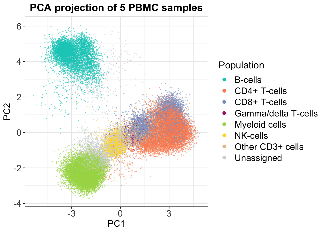
The problem is that PCA will likely only capture less than half of the total variance in the first two principal components, and another challenge is actually this linearity - it does not do well for most immune cell datasets (Chester & Maecker, 2015).

If we look at an example for 5 PBMC samples, in which populations were defined using manual gating, it is clear that the CD4+ and CD8+ T-cells are not separated in 2D. However, we do get some insights — it seems that B-cells are more distinct from the rest of the cell types.

2.1.2 t-SNE

t-distributed Stochastic Neighbor Embedding (t-SNE) was presented in van der Maaten et al. (2008) but is more commonly known as viSNE (Amir et al., 2013) when used for CyTOF data. Please note that viSNE relies fully on t-SNE and it is just a name for the implementation as a GUI.

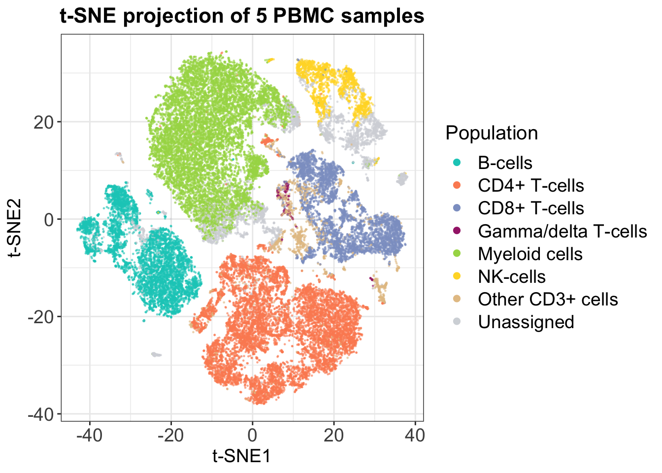
t-SNE is a ‘neighbor graph’ tool, which means that it relies on a completely different approach to dimensionality reduction. What it does is to quantify distances between each cell and its closest neighbors and preserves these, while distorting the global distances in its output. Therefore, you can not use distances between clusters in a t-SNE plot or count on the cluster sizes as a measure of variability, but the approach is conversely better at grasping high-dimensional patterns and at separating different populations completely. This is also seen in the following plot, which represents the same data as shown with PCA.

t-SNE is not as fast as PCA and its speed unfortunately scales poorly for large datasets. Furthermore, it is not possible to project new data into an existing t-SNE embedding, and you have to be careful with initialization, since t-SNE starts randomly by default. However, this last disadvantage is easily overcome in any programming language by setting the ‘seed’. Finally, t-SNE does not allow duplicate data points, i.e. two identical cells, and these must be removed before running. Because of these limitations, the use of UMAP in CyTOF analysis is expected to increase rapidly.

2.1.3 UMAP

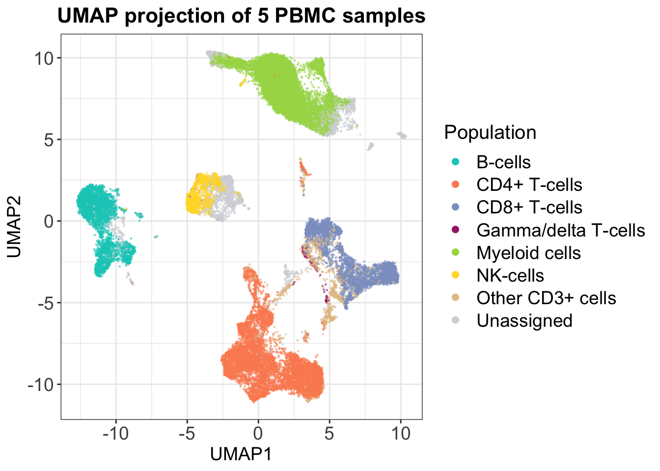
Uniform Manifold Approximation and Projection (UMAP) was first introduced for CyTOF data by Becht et al. (2018). This approach to dimensionality reduction also relies on information of a cells neighbors and is non-linear like t-SNE, but it yields much better preservation of the global data structure - distances between clusters are actually somewhat meaningful. This is also highlighted by the plot below, which again depicts the same set of cells as for PCA and t-SNE. We notice that all the T-cell types are separated but that they closer together than the rest of the clusters. Like the PCA, we again see that B-cells are highly separated from the rest on the second axis, and we also observe that the individual cluster shapes in the UMAP are somewhat similar to the t-SNE plot. This simple example highlights that UMAP preserves local and global structures of high-dimensional data well.

UMAP provides faster runtimes for larger datasets than t-SNE, because the time scales linearly with the number of cells, and like PCA, it is actually possible to project new cells into an existing UMAP. Like t-SNE it has a random start, which again can be fixed for reproducibility.

2.1.4 Dimensionality reduction speed

In the above sections we touched upon the fact that these methods have different runtimes. With small datasets the differences do not really matter because we will hardly notice the difference between ten seconds and one minute, but if we scale up to one day vs. six days we are definitely interested in this difference. Accordingly it is relevant for anyone to keep the estimated runtime of a method in mind when choosing an analysis approach — at the very least it can save you some frustration in the late hours of the night when you have a 9 o’clock presentation the next day if you know which methods are feasible to run in due time.

We compared PCA, t-SNE and UMAP runtimes for a CyTOF dataset with 20 channels using R implementations of each of the tools. The results are displayed in the graph below and it is very clear that PCA is by far the fastest method.

Runtimes for dimensionality reduction methods in R. For t-SNE, the Rtsne package and default settings were used, for UMAP, the umap package and settings: n_neighbors = 15, min_dist = 0.2, metric = ‘euclidean’, method = ‘naive’, and for PCA simply the base command prcomp. All methods were run on a single node with 24 cores and 256 GB RAM (two Intel E5-2680 CPUs).

2.2 Cell subset detection (clustering)

In the analysis of CyTOF data it is not uncommon to have millions of cells, making it impossible to study each individual cell one at a time. Additionally, it is important to remember that the immune system consists of millions and millions of cells and that a phenotypic change in tens of cells will not represent an actual change in the body. Stimuli such as infection or vaccination will lead to a large expansion of certain subsets of cells, which is detectable if one knows how to distinguish the given subset from the other cells. Immunologists have studied immune responses for decades and several approaches to identify subsets of interest have been invented, including manual gating that is conducted in a series of steps.

While application of that approach has greatly improved our understanding of the immune response, it also has drawbacks and as an alternative, clustering tools are being developed with CyTOF data in mind. There are several good reasons why we should switch to using these. First, you can get populations you would have missed in hand-gating. Particularly, subsets of the same cell type which you may only have known as a single group before but which actually shows a large degree of heterogeneity. Detecting such populations with clustering is possible because it is not limited to using two channels at a time but instead works in the multi-dimensional space that CyTOF data actually exists in. This enables clustering to detect much more complex data patterns. Other advantages for clustering compared to hand-gating is reproducibility and to some degree speed — or at least less manual work. However, cluster annotation is still a manual process.

One challenge that occurs in the use of clustering for CyTOF analysis is the fact that it does not always yield results which are compatible with current biological understanding or manual gating. Accordingly, the jump into using these approaches may seem troublesome and even terrifying. The reason why results from the two methods differ is that clustering detects mathematical patterns in the data and humans do not. Because of experience, humans have a strong bias towards known patterns; the (unsupervised) clustering approaches however, attacks the problem completely naively. This can mean that clustering comes up with biologically nonsensical results — or at least we think they do. However, one must remember that the results of clustering are mathematically correct and our best recommendation would be to stay critical and utilize your experience in immunology while also keeping an open mind towards ‘odd-looking’ clustering results as these may truly contain relevant — and perhaps previously unknown — cell subsets.

A number of clustering tools exist and to further the incorporation of these in CyTOF data analysis we have described some of the commonly used tools below. Remember that you may want to use more than one of these and that you can also use them more than once on the same dataset (i.e. first define one subset out of all cells and then re-cluster that subset to search for more subtle distinctions).

2.2.1 FlowSOM

FlowSOM was originally developed by Van Gassen et al. (2015) and is a tool for detection of groups of cells with similar features. The main advantage is the method’s speed, since this makes it possible to run the clustering of cells using all the events in a dataset (see also clustering speed section). This method is also highlighted as one of the best-performing by Weber & Robinson (2016). What drives the high speed of the method is that the tool uses a so-called self‐organizing map (SOM). This method of clustering relies on automatic detection of data patterns (i.e. distinct cell groups) starting from a random initialization.

A 2D example of a self-organizing map with two neurons is illustrated below. In the case of FlowSOM it is possible to define both the number of neurons (default = 100) and the channel/markers to use for generating the SOM. This means that the input would be an expression matrix including all markers of relevance, and the output would be the so-called “codebook” that each event belongs to.

However, it does not end at the generation of the SOM. FlowSOM actually utilizes so-called meta-clustering after the initial map is made. In this process, the codebooks are grouped into a defined number of meta-clusters, which serve as the output of the tool. This number of meta-clusters in the output must be defined by the user. This can bias the results, and one should preferably explore the results with different numbers of clusters to see what works for a given case. In general, it is recommended to set the amount of meta-clusters to a larger number than what is to be expected and then manually merge clusters in the downstream analysis based on biological knowledge.

An advantage in using clustering is, as mentioned, that you get a large degree of reproducibility. This is achieved in FlowSOM by making sure that the random initialization is the same every time and in practice it is ensured by fixing the seed of the algorithm. Additionally, there are approaches to avoid having to choose the number of meta-clusters yourself (e.g. the elbow method), which we will not describe in detail here. Another advantage is that it is very easy to check results with different numbers of meta-clusters, since the computer does all the work for you. Generally, it is always recommendable to run a clustering tool with random elements a couple of times to check the stability of the results - firstly, ‘unfortunate’ initializations can lead to a signal in the data being lost due to random chance and secondly, stability indicates a strong biological signal.

The FlowSOM tool also comes with visualizations that can be used for cluster annotation including minimum spanning trees. An example of the output is shown in the hierarchies section. The tool has no graphical user interface, but is implemented as a package for the R programming language. The tool was applied in Guilliams et al. (2016) and Collier et al. (2017) for analysis of flow cytometry data, and in Krieg et al. (2018) for analysis of mass cytometry data.

Since FlowSOM incorporates all cells in the definition of its clusters, it is important to include all the samples you want in an analysis when actually running FlowSOM as there is no easy way of adding new data to an existing clustering. Of course you can cluster the new data separately and try to match the clusters across your runs, but it will never be the same as having all your data in a single run. Therefore, it is often an advantage to include all your data at first, perform clustering, and then simply leave out some samples from further analysis. Imagine a case where your initial data contains five subpopulations, and the data you want to add later contains seven. If you try to map the new data into the clusters of the initial data you will have problems. The only reason to start with a subset of your data would be a case where more subtle differences might get lost in the bigger picture of including all samples — something which is rarely the case. If in doubt, one can try both including and not including all data and see how it affects the results.

2.2.2 PhenoGraph

PhenoGraph was first presented by Levine et al. (2015) and is another method for clustering of cells in to smaller subsets based on the expression of selected proteins. It is supposed to perform well with several different types of cytometry data (Weber & Robinson, 2016).

Briefly, the tool works by constructing a ‘nearest neighbor graph’, which is built by detecting the N closest neighbors for each cell based on marker expression. Subsequently, the tool defines clusters as neighborhoods with a large degree of interconnectivity. This should allow the method to capture both rare and frequent cell types. The tool includes automatic detection of the number of clusters, however, the number of neighbors, N, to use must be defined by the user. The original paper suggests this to have little effect in the range N = 15-60 but we suggest to test a couple of options before choosing your own setting.

Furthermore, it is debatable whether it is an advantage that the algorithm detects the number of clusters itself. One can argue that it is less biased, but the counter-argument presented by Weber & Robinson (2016) is that it is better to leave the user in control since there is no right number of clusters because hematopoietic cells exist in a continuum. Nonetheless, PhenoGraph chooses for you.

PhenoGraph itself does not include any visualization but following clustering, a common visualization technique is to plot the cells colored by cluster in either a PCA/t-SNE/UMAP plot. Of course, a challenge that remains and which is not addressed by PhenoGraph itself is then to annotate the clusters. One approach for this is shown in the figure below.

2D t-SNE with PhenoGraph clusters displayed next to the same plot colored by expression of lineage markers. Data from a single PBMC sample of a healthy person. Notice that results are very comparable to those of FlowSOM and SPADE.

PhenoGraph was used for analysis of single-cell RNA-seq data in Keren-Shaul et al. (2017) and flow cytometry data in DiGiuseppe et al. (2017).

While the original developers of PhenoGraph suggest a method for matching clusters between samples and therefore encourage users to run one sample at a time, this is not the approach we would recommend. Instead we suggest that you run clustering of all samples together because it makes downstream analysis easier. PhenoGraph is one of the faster clustering methods making this feasible (see clustering speed section).

2.2.3 X-shift

X-shift was originally presented by Samusik et al. (2016) and has since been applied in several studies including Porpiglia et al. (2017) and Ajami et al. (2018). It essentially works by measuring how dense the surroundings of each cells are and looking for local peaks, such that these peaks constitute the cluster centroids. After centroids are defined, cells are added to the clusters based on proximity. Density is quantified based on the distance between a given cell and its nearest neighbors — and distance is measured in the space spanned by expression of user-selected markers.

This method does not require the user to input the number of desired clusters, and it also has a way of selecting how many neighbors to include in the density estimates, which should ensure that the true number of distinct populations is identified.

In the original article, results are primarily visualized using a plot of what is commonly known as a ‘decision tree’. Generally, you start with a cluster containing all cells, and then ask a question regarding the expression level of one of your proteins - e.g. ‘is expression of CD19 smaller than 1?’. For this question, you will then split your data in two — the cells whose expression of CD19 is equal to or greater than 1 (likely to your B-cells), and the rest. For the two resulting groups, you can ask a new question regarding another (or the same) protein. You repeat this until you end up with clusters that are relatively pure, i.e. they contain very similar cells. In the case of X-shift’s built-in visualization, you ask questions until you have a visualization that contains your pure clusters. This is very similar to the process of manual gating, and method behind the resulting plot should be very familiar to cytometrists.

Decision tree example.

The tool was built in Java, and it comes with a graphical user interface which should allow for easy data processing for all. There are some settings, which require a bit of thinking and decision-making including the distance measure and how many runs, you wish to go through to select the number of neighbors to use. Once again, the best recommendation is to test some different settings and see what works for you.

Tree illustrating clustering of a healthy PBMC sample. The number of clusters is 14 and the labels show which expression values are contained within the clusters. The coloring is based on expression of CD3. Cluster sizes are proportional to the size of each circle. From the plot, we clearly have CD4+ T-cells in clusters 10-11 and CD8+ T-cells in clusters 13-14. NK-cells are found in cluster 9, and B-cells in cluster 7. Myeloid and other cell types are spread across the remaining clusters.

This method was highlighted as the best method for detection of rare cell populations by Weber & Robinson, 2016. Unfortunately, the method is rather slow as seen below, and the same review suggests FlowSOM as a reasonable alternative. Of course, it is possible to perform downsampling before running but this is unadvisable when you wish to detect rare populations since you might end up discarding them completely.

2.2.4 ClusterX

The ClusterX tool was introduced as part of the R-package Cytofkit by Chen et al. (2016). This tool is accessible to non-coders as it comes with a graphical user interface, but it can also be run directly in R. This tool is among the slowest presented here and the package documentation actually recommends downsampling. This is not optimal, especially in terms of detecting rare populations. Cytofkit also contains implementations of DensVM, FlowSOM, and Phenograph.

ClusterX does not work directly on the multi-dimensional CyTOF data, but instead clusters cells based on a dimensionality-reduced projection of the data. Overall, the method consists of four steps: 1) Make a dimensionality-reduction (i.e. t-SNE/PCA/ISOMAP) map of the CyTOF data, 2) Estimate density at each point, 3) Detect density peaks, and 4) Assign clusters based on peak presence. The number of clusters is detected automatically using this approach.

This approach to clustering is extremely easy to grasp from a visual stand-point, but it definitely also has critical points: It seems counter-intuitive to work hard in the lab to generate high-dimensional data and then perform analysis based on dimensionality reductions. In any dimensionality reduction some information is inevitably lost and therefore it should be better to cluster in higher-dimensional space if one wishes to fully grasp the data. Furthermore, downsampling will be necessary for most datasets which, as discussed previously, is often a problem. All in all, spending time and money on generating data for as many cells with as many channels as possbile is not really rewarded in ClusterX. Furthermore, the authors show that ClusterX has a reasonable performance but this is not replicated in Weber & Robinson (2016).

2.2.5 SPADE

The SPADE method was presented by Qiu et al. (2011), and used for analysis in Bendall et al. (2011). Simply put, the method aims at identifying subsets of cells with similar protein expression, and it does so by performing ‘agglomerative clustering’, which is a type of unsupervised, hierarchical clustering (see below for details).

However, because this type of clustering is relatively slow, and most mass cytometry experiments yield many cells, the tool usually incorporates a subsampling of the total events. However, this is done while regarding density of the data points in order to preserve rare cell types for the clustering step. But of course, this can limit the quality of the analysis, since some patterns could be missed.

After performing the clustering itself, a visualization is made using a so-called minimum spanning tree. The name actually accurately describes the approach - it is the shortest possible path which connects all the derived clusters. The final part of the tool maps all the cells excluded from clustering back to the generated tree and assigns clusters to each cell. Lastly, the median protein expression for the included set of markers is calculated using all cluster members. The resulting visualization is good for studying the relationship between different cell types.

SPADE was actually updated twice to yield versions 2.0 and 3.0 (Qiu, 2012 and Qiu, 2017), and the current implementation is deterministic (i.e. it provides the same result every time - despite using downsampling). It is a MATLAB-based tool which comes with graphical user interface allowing for easy usage by non-programmers.

An example of the output for a PBMC sample of a single healthy person is shown below. The results are largely comparable to those from FlowSOM.

Minimum spanning tree illustrations of SPADE results. Each cluster is represented by a circle. All the small plots show expression of the clustering markers, and the large plot shows a manual cluster annotation based on protein expression.

SPADE was one of the first tools directed at CyTOF data but in a comparison by Weber & Robinson (2016) it showed very poor performance in terms of replicating manual gating. The main advantage is that the method is relatively fast and it may provide a good initial overview of the main populations in a dataset.

2.2.6 Clustering speed

The time it takes for each of these clustering algorithms to run is actually a major component in how you end up analyzing your CyTOF data. This is because some methods require downsampling to run at all and others may simply take days to run for your data. Therefore, it is key to keep in mind approximately which runtime you can expect so you adjust your expectations and execution accordingly! You may be fine with running FlowSOM for 15 minutes on your laptop, but it you are planning to execute an algorithm which takes a day you may want to use a server. Consequently, this section is dedicated to the presentation of some runtimes - and how they scale.

Weber & Robinson (2016) also test runtimes in their analysis of clustering approaches and below we have simply tried to summarize their results in a plot:

Please note that not all hyperparameters are the same and that there are different numbers of dimensions in the datasets. However, this should give you an idea of runtimes and whether subsampling is necessary (notice the log-transformed y-axis). When there is ‘missing’ datapoints in the above plot it is because the authors chose to downsample due to large runtimes.

The datasets in the above comparison were however quite small (up to 10 samples) and as a consequence we updated this analysis:

Clustering runtimes for FlowSOM as a function of the number of included cells using 20 channels. MC = meta-clustering.

With constant settings regarding the number of included channels (20), FlowSOM’s runtime scales completely linearly (R² = 0.999) with dataset size, and meta-clustering is pretty much running in constant time. FlowSOM’s estimated runtime for an astonishing 100,000,000 million cells with 20 channels is therefore only 5 hours and with the current pre-processing pipelines, this runtime will never be the bottleneck of the analysis. Even if adding 40 channels, which is not advisable as this would correspond to all channels in most CyTOF dataset, the runtime will still be less than 10 hours and completely manageable (especially on a server) as illustrated by the graph below.

Clustering runtimes for FlowSOM as a function of the number of included channels using a million cells. MC = meta-clustering.

2.3 Analysis of differential abundance of cell populations and proteins

2.3.1 Analysis of differential abundance of cells in clusters

2.3.1.1 cydar

cydar (Lun et al., 2017) was developed to study patterns of differential abundance in mass cytometry data. One can easily imagine this being a matter of great interest in several scenarios related to the immune system - i.e. if comparing a group of healthy individuals and a group of people infected with influenza virus, it could be expected that there would be a larger proportion of CD8+ cytotoxic T cells present in the infected individuals.

This tool analyses data in two main steps. First, cells are assigned to so-called ‘hyperspheres’. These hyperspheres are not mutually exclusive, and they do not represent cell types directly. They simply represent a group of cells with shared features. The second step, is to test for differential abundance between user-defined sample groups. Specifically, the method tests for differences in the relative count of a hypersphere. After obtaining the initial results, the actual biological results have to be derived manually, by studying the protein expression in the hyperspheres with differential abundance.

cydar example. Most hyperspheres turned out to have decreased abundance in the treated samples (blue), and the cells in these hyperspheres are distinguished by being negative for Marker B. For the few upregualted hyperspheres, there appear to be two main clusters - one of which is positive for Marker A (yellow).

cydar is a diverse tool, which can account for relatively complex study designs such as those encompassing paired samples and time-course studies. However, this flexibility comes at a cost, since the tool is not available as a graphical user interface. A use case is presented by Richard et al. (2018).

2.3.2 Analysis of differential expression of proteins between clusters

2.3.2.1 Citrus

Citrus (Bruggner et al., 2014) was made with the purpose of detecting features that differ significantly between two or more experimental groups. These features may be either protein expression levels or cell type abundances, or both. Examples of experimental groups could be different treatments, different time points, or healthy vs. diseased. The tool is relatively easy to use even for non-coders as it comes with a graphical user interface.

The tool works by first performing clustering on the input data set, and then identifying differences between groups of samples. More specifically, Citrus performs unsupervised hierarchical clustering (see the extra notes section) using a subset of the total input cells (for computational efficiency, and to make sure each sample contributes equally to the pool of cells). This clustering is performed based on the expression of a set of user-defined markers, which will typically be those normally used for manual gating. Since the clustering is hierarchical, one should be aware that the clusters are not mutually exclusive and some cells will be present in more than one cluster. The central cluster (Number 1 on the figure below) contains all cells, Cluster 2 contains a subset of the cells in cluster 1, cluster 3 contains a subset of the cells in cluster 2, etc.

After clustering, Citrus tests for features that differ significantly between the user-defined sample groups, in each cluster. This is done using up to three different statistical models. For differential expression purposes, Citrus will test for differences in the median expression of each selected protein. Here, it is important to make sure that the data is ArcSinh-transformed before testing (possible to have Citrus do this), and one should not test for differential expression in markers, used for clustering. For differential abundance, the percentage of cells in a sample belonging to each cluster is considered.

The results of a Citrus analysis are mainly graphical. First, you may obtain an overview of the protein expression in each cluster, and then you can look for the specific features that are significantly associated with each experimental group. The results are presented for different levels of significance (based on q-values), which should essentially indicate how clear the difference is.

Citrus result example (simplified). Left: Expression of clustering markers in the derived clusters. The results highlighted that Marker C was differentially expressed in the double-positive clusters (circled), and looking specifically at the level of expression in the red arrow cluster, it turned out that the untreated group displayed higher levels of Marker C than the treated group.

A couple of caveats to keep in mind is that Citrus is not reliable when clusters are too small - and consequently, the user should define a minimal cluster size allowed. Additionally, at least eight samples should be in each experimental group for reliability of the results. The method in itself is not suitable for time-course data with three or more time-points. Finally, it is important to note that the use of median expression levels may be misleading in some cases, but it is generally a decent approximation.

An example of Citrus being used is presented in Gaudillière et al. (2014).

2.4 Cellular hierarchies

2.4.1 FlowSOM

FlowSOM (Van Gassen et al., 2015) was also described in the clustering section, but should also be considered a tool to study cellular hierarchies. Specifically, the tool can also serve to generate visualizations, which can be useful in the interpretation of results. This type of visualization is called a minimum spanning tree, and essentially connects each cluster to the most similar other clusters (as described for SPADE above). This allows users to understand how clusters relate and study hierarchies such as those in developmental studies. An example using a PBMC sample of a single healthy person is shown below.

This tree clearly shows distinct clusters with different biologically relevant features. Cluster 3 is characterized by expression of CD16 and CD56 and must represent NK-cells, cluster 6 (CD19+/HLA-DR+/IgD+) represents B-cells, and clusters 7 (CD3+/CD4+) and 8 (CD3+/CD8+) contain T-cells. In this manner, it seems that all lymphocytes group together, and conversely, clusters 1 and 2 seem to represent myeloid cells with expression of CD11c, CD16, CD14, CD33, CD123, HLA-DR, and CD4 to various degrees. The results are largely comparable to those from SPADE.

Minimum spanning tree illustraion of FlowSOM results. Each cluster is represented by a circle. The background coloring represents the clustering, and the pie-like chart in each circle illustrates the protein expression in the cluster.

In mass cytometry studies, it is most useful to use only a subset of markers, when generating the tree as results can otherwise get confusing. After initial analysis, subsets of the cells can be separately analyzed.

2.4.2 Wanderlust

The Wanderlust method was developed by Bendall et al. (2014) and they used the method for studying human B-cell development. Essentially, this tool works by detecting which cells are most similar to a user-defined ‘start cell’, and then defines a path through all the cells to get to the cell most distant from the ‘start cell’. Because development is a continuous process, one should assume that many ‘in-between cell types’ are present in any developmental path, and these can be detected by having protein expression, which is a mixture of that of the sorrounding well-known cell types.

With the resulting trajectory, it should be possible to understand the order of certain developmental events, which end up determining the faith of the cells. Additionally, the tool could be helpful to place a previously unknown cell types relative to other well-studied types along the same developmental path. This can help elucidate the function of the type of cell.

The tool relies on certain assumptions: 1) The sample must contain cell types at all stages of development - also those that may be rare, 2) Protein expression changes occur gradually during development, and 3) No branching is present in the trajectory. The last of these is a problem for most hematopoietic cell types including T-cells, which branch into CD4+ or CD8+ cells. As a consequence, other tools including Wishbone (Setty et al., 2016) have been developed.

Currently, the official webpage for the tool is not running, but an R implementation exists.

3 Extra notes

3.1 What is “supervised” learning?

In supervised learning we have certain examples, for which we know both the input and output. E.g. we may have CyTOF data for 100 cells, 40 of which have been labeled as T-cells and 60 of which have been labeled as B-cells. We can then study these 100 cells and learn about the differences between the two cell types. We may discover that T-cells are negative for CD19 and positive for CD3, and the next time we see a CD19-/CD3+ cell, we will label it as a T-cell. The goal in supervised learning is to leverage existing pairs of inputs and outputs to make a model that can generalize for new examples, for which the output is not already known.

The presented example represents a classification problem, since there is a finite number of possible outputs in the ‘model’ (the output is discrete).

3.2 What is “unsupervised” learning?

In unsupervised learning, the data alone is used to learn the output values - there is no ‘right’ answer and it is therefore referred to as ‘exploratory analysis’. So what can be learned? Different things - but most commonly, we look for structure. Clustering is a method within unsupervised learning - we wish to divide data into meaningful groups based on the data structure. The goal is to define observations (i.e. cells) that share features (i.e. similar protein expression). It is the unsupervised counterpart to classification. How to define (dis)similarity then remains the question in more ways than one. Firstly, there are different distance metrics one can apply such as the Euclidean distance or other less well-known methods. Secondly, a challenge is generally to avoid ending up with too few or too many clusters - you want enough distinct clusters to learn about biological differences, but you do not want a thousand small clusters, some of which share almost all features anyway.

There are two main approaches to clustering, partitional and hierarchical clustering.

• In partitional clustering, the goal is to split the data into a fixed number of groups, which do not overlap. Example: B-cells and T-cells are different groups, and the members do not overlap. A cell can only be a member of one of these groups.

• In hierarchical clustering, you essentially start by having each point alone, and then merge more and more groups based on proximity, until everything belong to the same cluster (agglomerative clustering) - or vice versa (divisive clustering). This yields a tree-like structure, in which the groups are subsets of each other. As an example we may have a group of myeloid cells and a group of lymphocytes. The latter contains three subgroups; NK-cells, B-cells, and T-cells, and the T-cells can be grouped further into CD4+ and CD8+ cells etc. A CD8+ T-cell would then actually belong to three groupings: Lymphocytes, T-cells, and CD8+ T-cells.

3.3 ArcSinh-tranformation

The expression values of raw mass cytometry data have a particular distribution, and while most of the values are rather low (0-10), some values can be in the 100’s. This type of distribution makes it hard to visualize data and perform manual gating, and as a convention, it is therefore common to transform the raw values before any processing. This is typically done using the ArcSinh-function, which transforms small values linearly, while scaling down the larger values more drastically. Moreover, the raw data is usually divided by 5 (the co-factor) before transformation by convention. This dogma of transformations has spread to many of the tools presented on this site, and all of the tools on this page expect the input data to be transformed - or can do so themselves.

 

---

Contact