Phenotype transfer between CyTOF and scRNA-seq
Søren H Dam
Last updated on 2026-06-19
This vignette demonstrates integrating a split-sample scRNA-seq and CyTOF experiment (Su et al.). The purpose is to transfer phenotypes from the CyTOF annotation to the scRNA-seq data, thus automating its annotation. The hope is that this process will identify cell populations otherwise only found in the CyTOF dataset, although at the expense of not finding populations only found by manually annotating the scRNA-seq data. To assimilate scRNA-seq data to CyTOF, we use our own implementation of Single-cell nearest-neighbor pseudobulking (scennep).
Dependencies
## Loading required package: SeuratObject## Loading required package: sp##
## Attaching package: 'SeuratObject'## The following objects are masked from 'package:base':
##
## intersect, t##
## Attaching package: 'anndata'## The following object is masked from 'package:SeuratObject':
##
## Layers##
## Attaching package: 'dplyr'## The following objects are masked from 'package:stats':
##
## filter, lag## The following objects are masked from 'package:base':
##
## intersect, setdiff, setequal, unionlibrary("ggplot2")
library("patchwork")
library("cyCombine")
library("cyDefine") # Available at https://github.com/biosurf/cyDefine##
## Attaching package: 'cyDefine'## The following object is masked from 'package:cyCombine':
##
## batch_correctDownload data
We got the download instructions from the article’s Data availability section. CyTOF is available on FlowRepository (FR-FCM-Z6ZN) and scRNA-seq data is available on SRA (SRR23497303). Getting the scRNA-seq metadata took some looking around, but direct download links are presented in the code chunks.
Get CyTOF data (FR-FCM-Z6ZN)
FlowRepositoryR might be depricated, so manual download can be required.
Get scRNA-seq data (SRR23497303)
Run in bash.
cd ../../../data/pbmc/paired_cytometry_scrna/rnaseq

# SRA Normalized
#wget https://sra-pub-run-odp.s3.amazonaws.com/sra/SRR23497303/SRR23497303
# Raw bam file (used)
wget https://sra-pub-src-1.s3.amazonaws.com/SRR23497303/possorted_genome_bam.bam.1
mv possorted_genome_bam.bam.1 possorted_genome.bam

# Metadata
wget https://ftp.ncbi.nlm.nih.gov/geo/samples/GSM7048nnn/GSM7048570/suppl/GSM7048570%5Fpbmc%5Fseq.h5ad.gz
gunzip rnaseq/GSM7048570_pbmc_seq.h5ad.gz
rm rnaseq/GSM7048570_pbmc_seq.h5ad.gz
Preprocessing
Before I found the preprocessed data from the article, I manually rerun the preprocessing steps. In the end, I used my own preprocessing, but used their filtering. There is commented out code for reusing their expression data, if you are redoing the analysis and want to keep it simple.
scRNA-seq
First, I convert the bam file to fastq in order to reanalyze with Cell Ranger.
module load cellranger/9.0.1
module load bamtofastq/1.3.0

# Get reference
wget "https://cf.10xgenomics.com/supp/cell-exp/refdata-gex-GRCh38-2024-A.tar.gz"
tar -zxvf refdata-gex-GRCh38-2024-A.tar.gz

# Bam to fastq
bamtofastq --nthreads 38 possorted_genome.bam fastq
mv fastq/ES-PBMC-2_HiSeq_MissingLibrary_1_HJK5NBCX2/* fastq/.
rm -rf fastq/ES-PBMC-2_HiSeq_MissingLibrary_1_HJK5NBCX

# Cell Ranger
cellranger count --transcriptome refdata-gex-GRCh38-2024-A --fastqs fastq --localcores 39 --localmem 110 --output-dir cr_out --id cr_paired_rna --create-bam=false
Then, I load the output into Seurat for preprocessing.
seu <- Seurat::Read10X("../../../data/pbmc/paired_cytometry_scrna/rnaseq/cr_out/outs/filtered_feature_bc_matrix")
seu <- CreateSeuratObject(counts = seu, project = "paired_rna", min.cells = 3, min.features = 200)
seu[["percent.mt"]] <- PercentageFeatureSet(seu, pattern = "^MT-")

# VlnPlot(seu, features = c("nFeature_RNA", "nCount_RNA", "percent.mt"), ncol = 3)
(Commented out) I manually set the processing thresholds as follows:
# seu <- subset(seu, subset = nFeature_RNA > 250 & nFeature_RNA < 2800 & percent.mt < 5)
# VlnPlot(seu, features = c("nFeature_RNA", "nCount_RNA", "percent.mt"), ncol = 3)
I reused the filtering and annotation from Su et al.
# Load anndata
adata <- read_h5ad("../../../data/pbmc/paired_cytometry_scrna/rnaseq/GSM7048570_pbmc_seq.h5ad")
#
# # Access the data
# count_matrix <- adata$X
# seu <- Seurat::CreateSeuratObject(t(adata$raw$X))
# seu <- seu[, adata$raw$obs_names %in% rownames(metadata)]
# count_matrix <- count_matrix[adata$raw$obs_names %in% rownames(metadata), ]
metadata <- adata$obs
# gene_info <- adata$var

# seu <- subset(seu, subset = nFeature_RNA > 250 & nFeature_RNA < 2800 & percent.mt < 10)
# seu <- subset(seu, subset = nFeature_RNA > 250 & (nFeature_RNA < quantile(nFeature_RNA, .95)) & percent.mt < 10)
seu <- seu[, colnames(seu) %in% rownames(metadata)]

# rna <- tibble::as_tibble(count_matrix) |>
#   mutate(cell_id = rownames(count_matrix),
#          celltype = metadata$celltype)

seu <- AddMetaData(seu, metadata)
# seu$in_orig <- if_else(colnames(seu) %in% rownames(metadata), true = "In", false = "Not in")
Visualizing scRNA-seq
## Normalizing layer: counts## Finding variable features for layer counts## Centering and scaling data matrix## PC_ 1
## Positive: BCL11B, CD247, RORA, IL32, PPP1R16B, TRAC, TC2N, TNIK, RHOH, INPP4B
## CAMK4, LINC-PINT, ANK3, IL7R, PCED1B, BCL2, TRBC2, THEMIS, RPS12, RPS18
## LTB, PDE3B, LDHB, CD69, SYTL3, TTC39C, TRBC1, ZEB1, TAFA1, PATJ
## Negative: FCN1, PLXDC2, LYZ, IFI30, CST3, MNDA, LRMDA, SLC8A1, S100A9, AIF1
## CLEC7A, NAMPT, LST1, HCK, S100A8, ENSG00000257764, VCAN, CYBB, SPI1, DMXL2
## CLEC12A, CSTA, SLC11A1, RBM47, CSF3R, IRAK3, CTSS, SERPINA1, NCF2, TNFAIP2
## PC_ 2
## Positive: BANK1, IGHM, AFF3, FCRL1, LINC00926, CD79A, NIBAN3, COL19A1, IGHD, PAX5
## MS4A1, EBF1, GNG7, ADAM28, RALGPS2, CD79B, RUBCNL, CD22, ANGPTL1, BLK
## KHDRBS2, TCL1A, ADAM7-AS1, COBLL1, HLA-DQA1, BCL11A, OSBPL10, CDK14, LIX1-AS1, WDFY4
## Negative: S100A4, SRGN, CD247, TMSB4X, SYTL3, IL32, MYO1F, S100A6, RORA, AOAH
## ARHGAP26, NKG7, CCL5, TNIK, BCL11B, RAP1GAP2, ANXA1, TGFBR3, CTSW, GZMA
## SAMD3, CST7, ID2, PYHIN1, FNDC3B, GZMH, NEAT1, TRAC, HIVEP3, SLCO3A1
## PC_ 3
## Positive: NKG7, GNLY, GZMB, CST7, GZMA, FGFBP2, CCL5, AOAH, KLRD1, GZMH
## PRF1, MCTP2, C1orf21, ZEB2, KLRF1, CTSW, SPON2, RAP1GAP2, MYO1F, SYNE1
## HOPX, CCL4, LINC02384, FCRL6, PDGFD, PPP2R2B, NCALD, JAZF1, TTC38, VAV3
## Negative: PRKCA, CAMK4, SERINC5, LTB, LEF1, INPP4B, IL7R, RPL13, RCAN3, TSHZ2
## FHIT, RPS12, ANK3, MAL, NELL2, RPLP1, LDHB, RPS18, SESN3, ENSG00000249806
## MAML2, FAAH2, TESPA1, CCR7, PRKCQ-AS1, PAG1, BCL2, CSGALNACT1, PDE3B, PVT1
## PC_ 4
## Positive: HES4, ENSG00000287682, CDKN1C, FMNL2, CSF1R, LYPD2, FCGR3A, CCDC26, MS4A7, TBC1D8
## PAPSS2, TCF7L2, CTSL, IFITM3, BATF3, MS4A4A, CKB, LINC02345, KCNMA1, UICLM
## SPRED1, SIGLEC10, RHOC, HMOX1, NEURL1, VMO1, ICAM4, TNFRSF8, SCRN1, PELATON
## Negative: S100A12, VCAN, ENSG00000257764, CD36, S100A8, FCAR, CD14, CSF3R, MS4A6A, CREB5
## DYSF, AQP9, CXCL8, ENSG00000287979, CLEC4E, MGST1, LUCAT1, ACSL1, ANPEP, PLBD1
## CYP1B1, TEX14, THBS1, TREM1, CCDC200, ENSG00000289150, ENSG00000276216, NLRP12, S100A9, LINC00937
## PC_ 5
## Positive: RPS18, RPL13, RPS12, RPLP1, LINC-PINT, DPYD, JUNB, CD44, PPP1R16B, S100A6
## S100A4, RNF149, RORA, CRIP1, IL32, ARHGAP26, NEAT1, S100A10, NFKB1, ADGRE5
## FBXW7, NIBAN1, MYO1F, TNFAIP3, PICALM, SYTL3, CDC14A, JUN, GPCPD1, ANXA1
## Negative: PPBP, CAVIN2, PF4, GNG11, TUBB1, GP1BB, CMTM5, ITGA2B, ITGB3, NRGN
## H2AC6, CTTN, ENSG00000288882, SPARC, GP9, TREML1, ACRBP, CLU, MPIG6B, CD9
## SNCA, RGS18, BEX3, ENSG00000289621, MYL9, PRKAR2B, PGRMC1, TPM1, SH3BGRL2, MYLK## Computing nearest neighbor graph## Computing SNNseu <- FindClusters(seu, algorithm = 4, random.seed = seed)
# UMAP
seu <- RunUMAP(seu, dims = 1:10, seed.use = seed)## Warning: The default method for RunUMAP has changed from calling Python UMAP via reticulate to the R-native UWOT using the cosine metric
## To use Python UMAP via reticulate, set umap.method to 'umap-learn' and metric to 'correlation'
## This message will be shown once per session## 07:37:53 UMAP embedding parameters a = 0.9922 b = 1.112## 07:37:53 Read 2651 rows and found 10 numeric columns## 07:37:53 Using Annoy for neighbor search, n_neighbors = 30## 07:37:53 Building Annoy index with metric = cosine, n_trees = 50## 0% 10 20 30 40 50 60 70 80 90 100%## [----|----|----|----|----|----|----|----|----|----|## **************************************************|
## 07:37:53 Writing NN index file to temp file /var/folders/q4/05k1bf1x3jq6p6pm_5f1xnw40000gp/T//RtmpbxCIJG/file5c27336636ca
## 07:37:53 Searching Annoy index using 1 thread, search_k = 3000
## 07:37:53 Annoy recall = 100%
## 07:37:53 Commencing smooth kNN distance calibration using 1 thread with target n_neighbors = 30
## 07:37:54 Initializing from normalized Laplacian + noise (using RSpectra)
## 07:37:54 Commencing optimization for 500 epochs, with 104764 positive edges
## 07:37:54 Using rng type: pcg
## 07:37:56 Optimization finished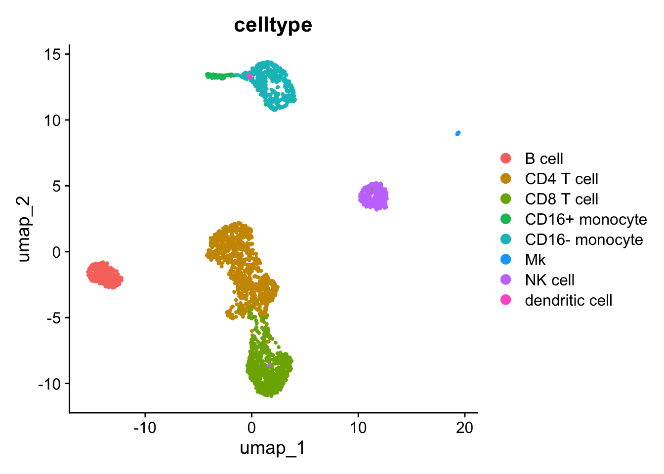
CyTOF
Load FCS files into R and clean marker names.
data_dir <- "../../../data/pbmc/paired_cytometry_scrna/FR-FCM-Z6ZN/"
cytof_fs <- cyCombine::compile_fcs(data_dir, pattern = "analyze_normalized")
## Reading 1 files to a flowSet..cytof_fs[[1]] |> flowCore::parameters() |> Biobase::pData() |>
dplyr::filter(stringr::str_detect(desc, "_"),
stringr::str_detect(desc, "BC", negate = T)) |>
pull("desc") ## $P2S $P3S $P12S
## "Event_length" "89Y_CD45" "115In_CD44"
## $P20S $P21S $P23S
## "141Pr_CD11b" "142Nd_CD79b" "144Nd_CD19"
## $P24S $P25S $P26S
## "145Nd_CD11c" "146Nd_IgD" "147Sm_CD68"
## $P27S $P28S $P29S
## "148Nd_CD16" "149Sm_CD25" "150Nd_CD43"
## $P30S $P32S $P34S
## "151Eu_CD103" "153Eu_CD45RA" "155Gd_CD27"
## $P35S $P36S $P37S
## "156Gd_CD86" "157Gd_Nucleoporins" "158Gd_CD33"
## $P39S $P40S $P41S
## "160Gd_CD14" "161Dy_Tbet" "162Dy_FoxP3"
## $P43S $P44S $P45S
## "164Dy_CD161" "165Ho_CD8a" "166Er_CD49a"
## $P47S $P48S $P49S
## "168Er_CD69" "169Tm_CD4" "170Er_CD3"
## $P50S $P51S $P52S
## "171Yb_CD20" "172Yb_CD38" "173Yb_CD45RO"
## $P53S $P54S $P55S
## "174Yb_HLADR" "175Lu_Perforin" "176Yb_CD56"
## $P57S $P58S $P59S
## "191Ir_Intercalator" "193Ir_Intercalator" "194Pt_Cisplatin"
## $P60S $P61S
## "195Pt_Cisplatin" "198Pt_Cisplatin"## Converting flowset to data frame## Extracting expression data..## Your flowset is now converted into a dataframe.## Transforming data using asinh with a cofactor of 5..## Done!colnames(cytof) <- colnames(cytof) |>
stringr::str_remove_all("^\\d+[A-Za-z]+_?")
cytof <- cytof[, stringr::str_detect(colnames(cytof), "^(CD|Fox|Tbet|id|sample|IgD|HLA)")]
markers <- cyCombine::get_markers(cytof)Annotation
I could not extract the annotation used in Su et al., so I manually annotated using more or less the same approach as they do.
cytof$label <- create_som(
  cytof, seed = 334, cluster_method = "flowsom", xdim = 6, ydim = 6, nClus = 18)

umap_cytof <- cytof |>
  plot_umap(markers = markers, col = "label", seed = 334, return_data = TRUE, down_sample = T, sample_n = 30000, title = "CyTOF UMAP")
## Generating UMAP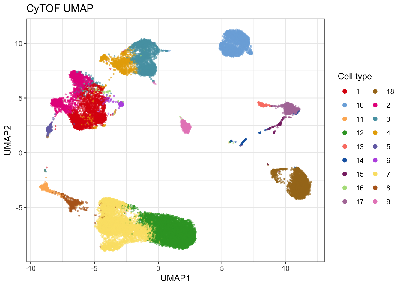
# plot_embedding(umap_cytof$data, col = "CD4", title = "CyTOF CD4")
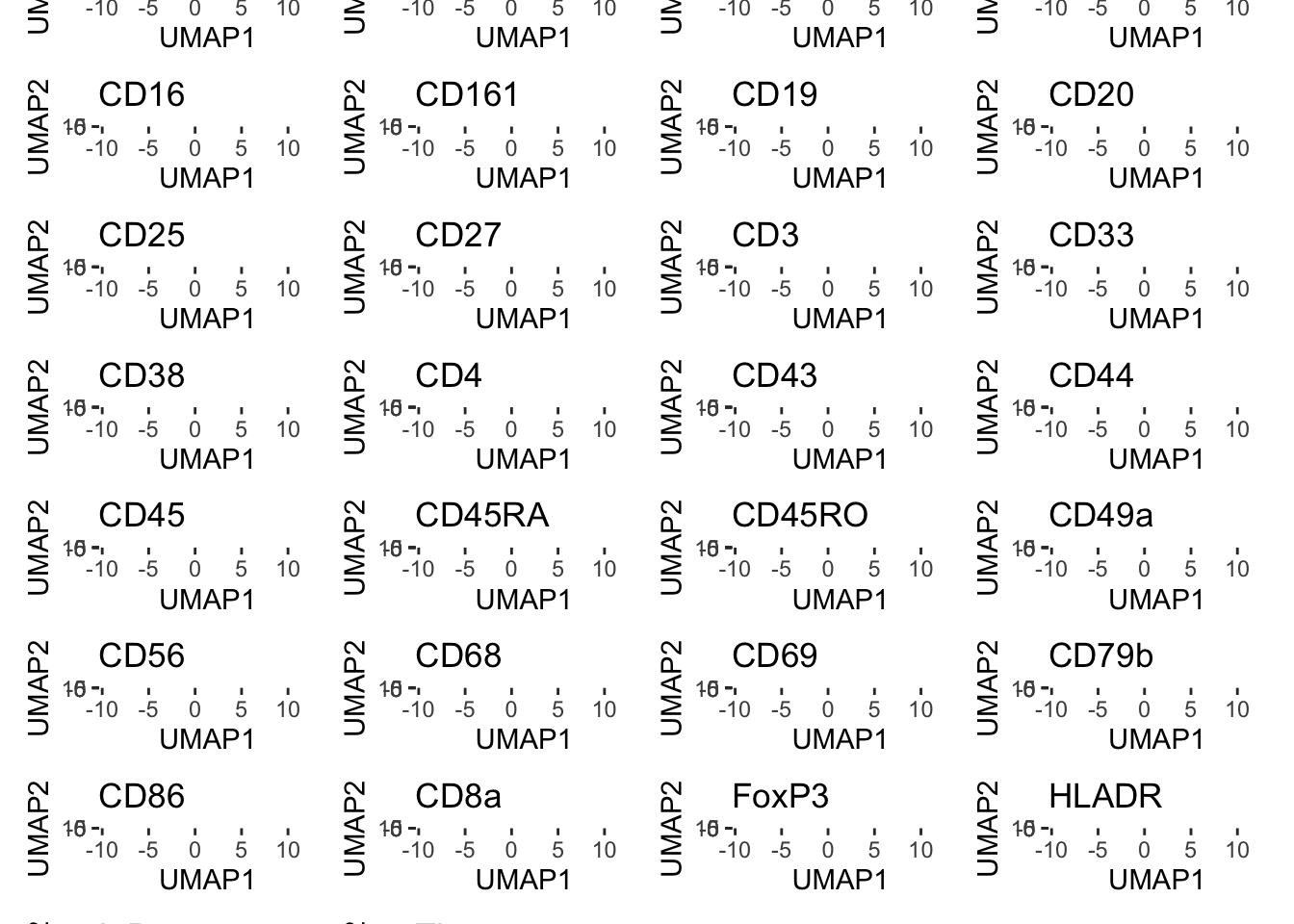
plot_markers(umap_cytof$data, markers = c("CD14", "CD16", "CD68", "HLADR", "CD3", "CD4", "CD8a", "CD19", "CD20", "CD56", "CD38"), show_legend = F)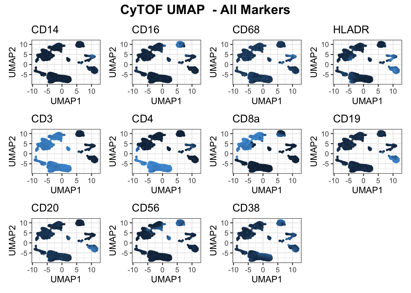
## Visualizing expression of predicted cell types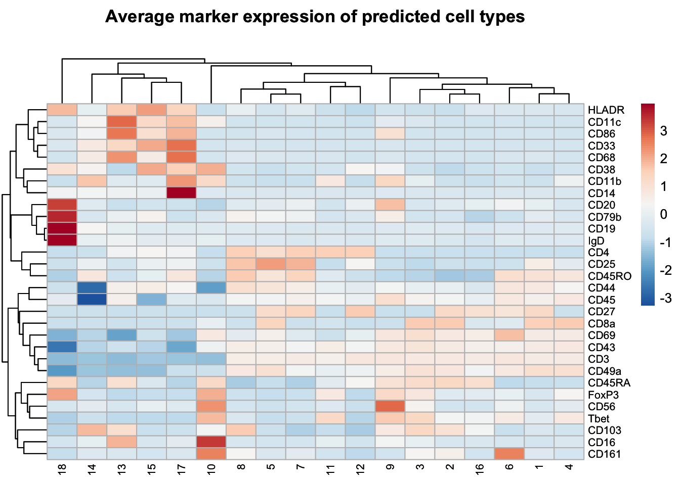
| Cell Type | Markers |
|---|---|
| CD4 T cells | CD3+, CD4+ |
| CD8 T cells | CD3+, CD8a+ |
| B cells | CD19+, CD20+, CD79b+, HLADR+ |
| NK cells | CD56+ |
| NKT cells | CD56+, CD3+ |
| CD16- monocytes | CD14+, CD16- |
| CD16+ monocytes | CD16+ |
| DCs | HLADR+, CD68+ |
| DN T cells | CD3+, CD4-, CD8a- |
| DP T cells | CD3+, CD4+, CD8a+ |
annotation <- c(
  "1" = "CD8 T cell",
  "2" = "CD8 T cell",
  "3" = "CD8 T cell",
  "4" = "CD8 T cell",
  "5" = "DP T cell",
  "6" = "DN T cell",
  "7" = "CD4 T cell",
  "8" = "CD4 T cell",
  "9" = "NKT cell",
  "10" = "NK cell",
  "11" = "CD4 T cell",
  "12" = "CD4 T cell",
  "13" = "dendritic cell",
  "14" = "unassigned",
  "15" = "dendritic cell",
  "16" = "DN T cell",
  "17" = "CD16- monocyte",
  "18" = "B cell")

cytof <- cytof |>
  mutate(label = stringr::str_remove_all(label, "cluster_"),
         batch = "CyTOF",
         celltype = annotation[label])

umap_cytof$data$celltype <- annotation[stringr::str_remove_all(umap_cytof$data$label, "cluster_")]

unique_cells <- c(as.character(seu$celltype), cytof$celltype) |> unique() |> sort()
celltype_colors <- cyDefine::get_distinct_colors(unique_cells)
celltype_colors["dendritic cell"] <- "#AA0A0A"

plot_cytof_exprs <- plot_embedding(umap_cytof$data, col = "celltype", title = "CyTOF", colors = celltype_colors, legend_title = "Cell type")
plot_cytof_exprs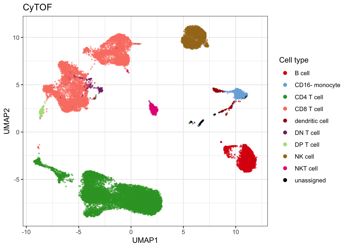
Convert protein to gene
I convert protein names to gene names to find the common features between the two datasets.
protein_gene <- data.frame(
  Protein = c("CD45", "CD11b", "CD79b", "CD11c", "IgD", "CD16", "CD25", "CD43", "CD103", "CD45RA",
              "Tbet", "FoxP3", "CD161", "CD8a", "CD49a", "CD3", "CD20", "CD45RO", "HLADR", "CD56"),
  Gene_Symbol = c("PTPRC", "ITGAM", "CD79B", "ITGAX", "IGHD", "FCGR3A", "IL2RA", "SPN", "ITGAE",
                 "PTPRC", "TBX21", "FOXP3", "KLRB1", "CD8A", "ITGA1", "CD3E", "MS4A1", "PTPRC",
                 "HLA-DRA", "NCAM1")
)


if ("CD45RO" %in% colnames(cytof)) {
  cd45 <- pmax(cytof$CD45, cytof$CD45RA, cytof$CD45RO)
  cytof <- cytof |>
    select(-starts_with("CD45")) |>
    mutate(CD45 = cd45)
  markers <- get_markers(cytof)
}

genes_to_rename <- rownames(seu)[rownames(seu) %in% protein_gene$Gene_Symbol]
rownames(seu)[rownames(seu) %in% genes_to_rename] <- protein_gene$Protein[match(genes_to_rename, protein_gene$Gene_Symbol)]
Run scennep
I run single-cell nearest-neighbor pseudobulking (scennep) using cosine distance. The umap demonstrates the impact of running scennep on the data.
## Run scennep
library(scennep)
rna <- scennep(
  seu,
  markers = markers,
  mc.cores = 4,
  distance = "cosine",
  return_S4 = FALSE
)
## Using the top 31 pcs for the SNN## Building SNN graph with k = 20## Pseudobulking each cell with its 20 nearest neighborsMerge datasets
seed <- 447
rna <- as.data.frame(t(rna))
rna$celltype <- seu$celltype
rna$batch <- "RNA"
rna$sample <- "RNA"
cytof$batch <- "CyTOF"


# Merge datasets
set.seed(seed)
uncorrected <- rna |>
  dplyr::select(dplyr::any_of(c(markers, non_markers))) |>
  dplyr::bind_rows(cytof |>
                     dplyr::select(dplyr::any_of(c(markers, non_markers)))) |>
  dplyr::mutate(id = dplyr::row_number())
Uncorrected
set.seed(seed)
uncor_batch <- uncorrected |>
  dplyr::group_by(sample) |>
  dplyr::slice_sample(n = nrow(rna)) |>
  plot_umap(
  down_sample = F,
  title = "Uncorrected",
  legend_title = "Technology",
  metric = "cosine",
  markers = markers,
  col = "batch")
## Generating UMAP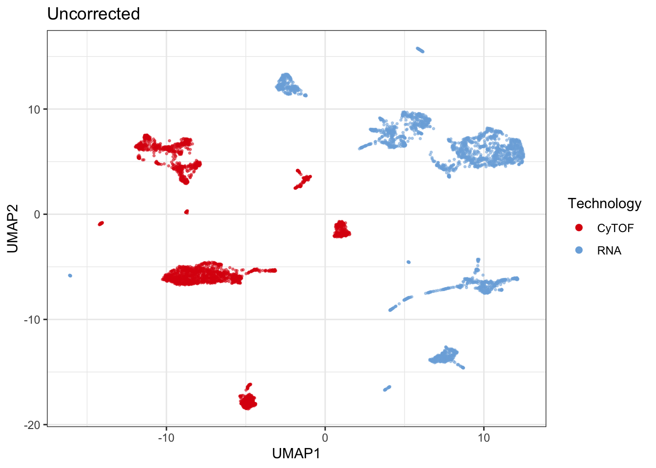
Batch correct
system.time({
  suppressMessages({ # Hide per-cluster correction info
    corrected <- cyCombine(
      uncorrected,
      markers = markers,
      norm_method = "scale",
      cluster_method = "flowsom",
      distf = "cosine",
      # ref.batch = "CyTOF",
      seed = seed,
      xdim = c(1, 5),
      ydim = c(1, 5),
      mc.cores = 4,
      method = "ComBat"
    )
  })
})
Plot results - Batch
set.seed(seed)
plot_batch <- corrected |>
  dplyr::group_by(sample) |>
  dplyr::slice_sample(n = 10000) |>
  plot_umap(
  down_sample = F,
  markers = markers,
  title = "CyTOF + scRNA-seq",
  return_data = T,
  metric = "cosine",
  legend_title = "Technology",
  col = "batch")
## Generating UMAP# ggplot2::ggsave(plot_batch$plot, filename = "figs/05_cytof_rnaseq_batch.png")
# saveRDS(plot_batch$plot, "results/05_cytof_rnaseq_batch.rds")
plot_batch$plot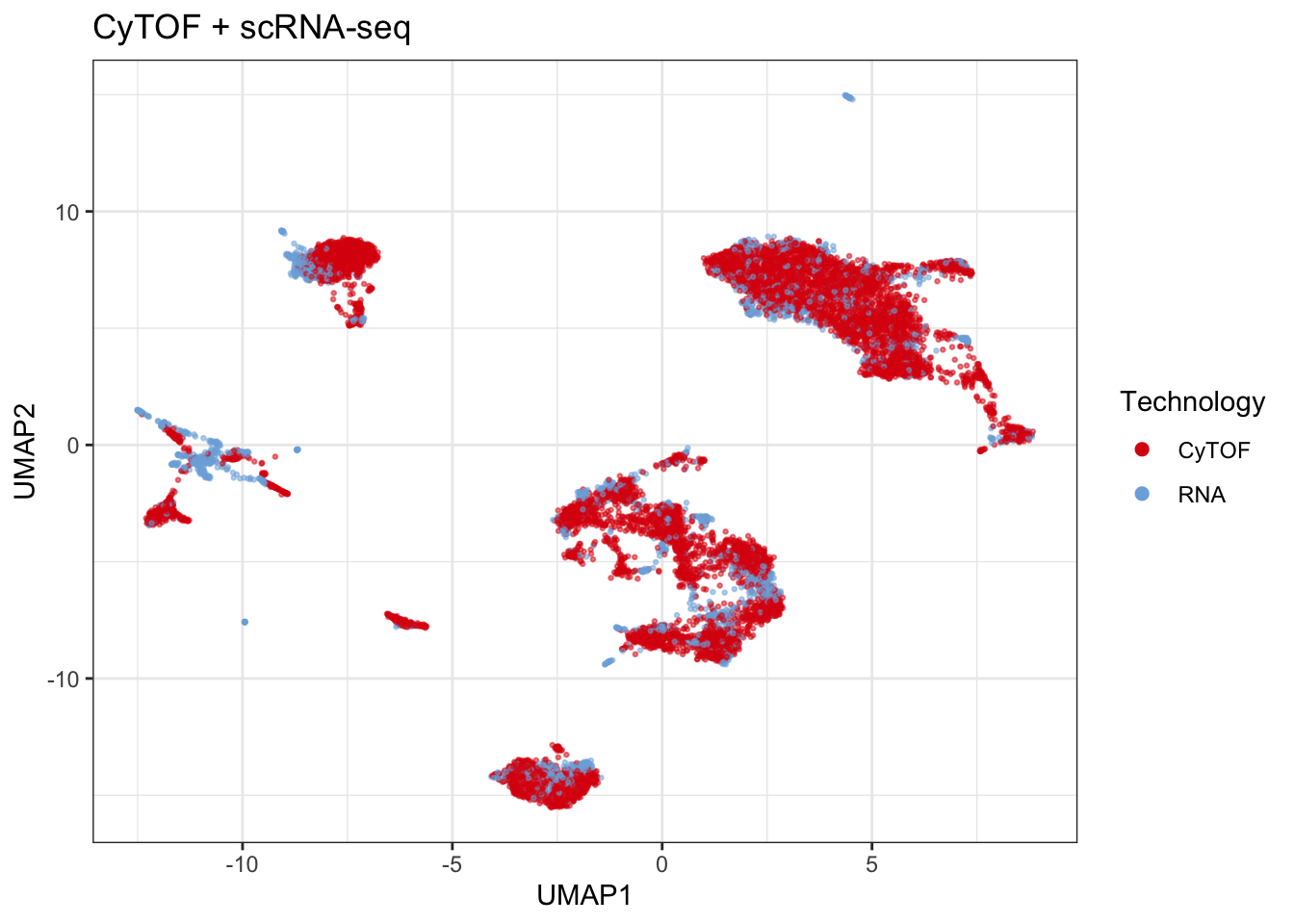
Plot results - Cells
Here, I reuse the umap generated above to plot celltype labels on the two modalities side by side.
xlim <- c(min(plot_batch$data$UMAP1), max(plot_batch$data$UMAP1))
ylim <- c(min(plot_batch$data$UMAP2), max(plot_batch$data$UMAP2))

plot_cell <-
  plot_embedding(
    dplyr::filter(plot_batch$data, batch == "CyTOF"),
    colors = celltype_colors,
    xlim = xlim,
    ylim = ylim,
    title = "Integrated CyTOF",
    col = "celltype",
    legend_title = "Cell type") +
  plot_embedding(
    dplyr::filter(plot_batch$data, batch == "RNA"),
    colors = celltype_colors,
    xlim = xlim,
    ylim = ylim,
    title = "Integrated scRNA-seq scennep",
    col = "celltype",
    legend_title = "Cell type") +
  patchwork::plot_layout(
    axes = "collect",
    axis_titles = "collect")

plot_cell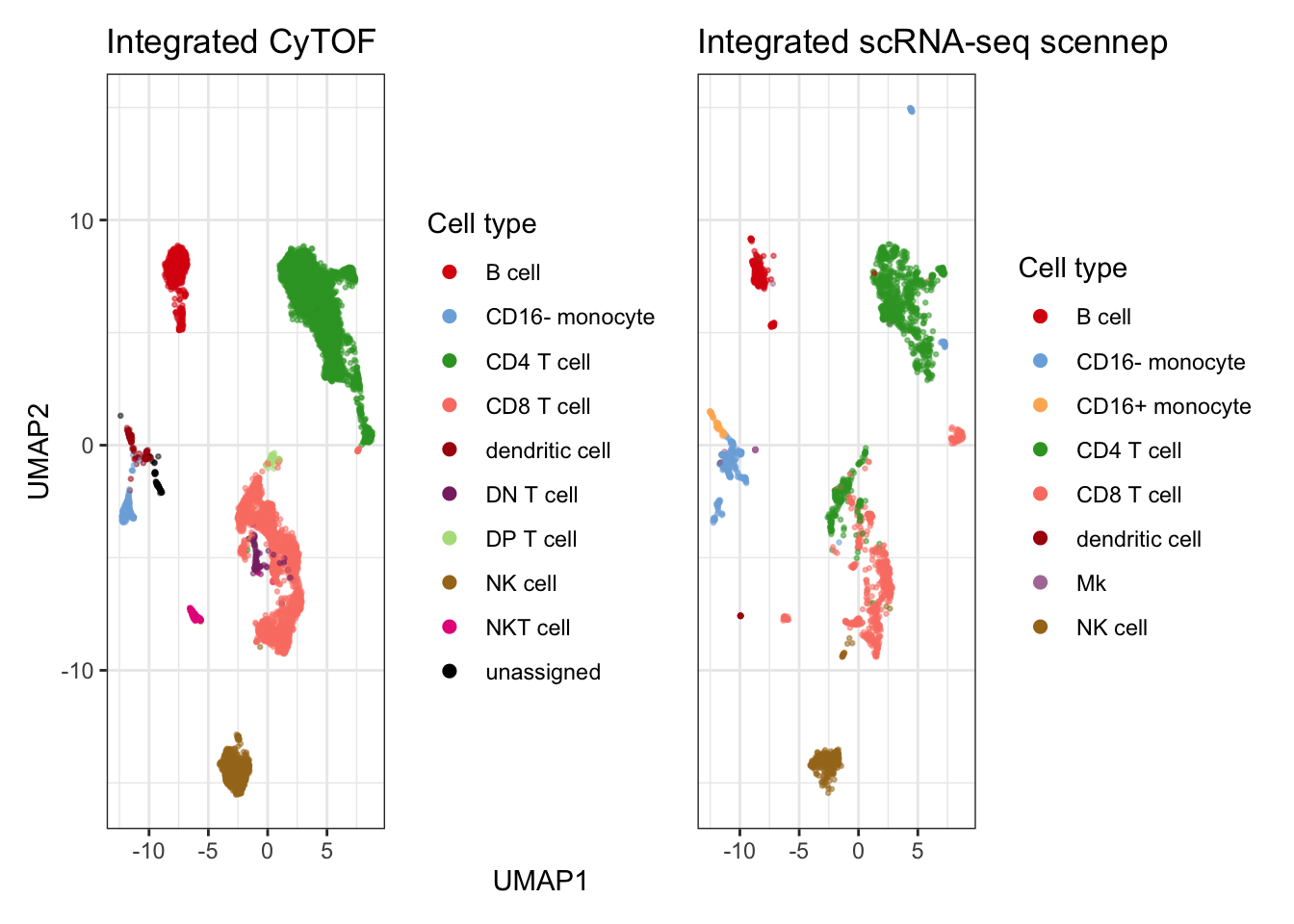
Phenotype transfer with cyDefine
markers <- cyCombine::get_markers(corrected)
classified <- cyDefine::cyDefine(
  corrected |> dplyr::filter(batch == "CyTOF"),
  corrected |> dplyr::filter(batch == "RNA"),
  markers = markers,
  using_pbmc = FALSE,
  adapt_reference = FALSE,
  batch_correct = FALSE,
  seed = seed,
  identify_unassigned = TRUE,
  train_on_unassigned = FALSE,
  mtry = 10,
  num.threads = 4,
  num.trees = 1000
)
## Training random forest model using 4 threads## Model training took 3.17 seconds## Predicting..## Classification took 3.79 seconds## Outlier detection took 0.01 secondsFigure 4A - UMAP
colors <- cyDefine::get_distinct_colors(sort(unique(classified$reference$celltype)), add_unassigned = TRUE)
p_umap <- plot_umap(
    classified$reference,
    classified$query,
    markers = markers,
    colors = colors,
    ref_col = "celltype",
    query_col = "predicted_celltype",#"model_prediction",
    build_umap_on = "reference",
    title = c("Reference (CyTOF)", "Query (scRNA-seq)"),
    seed = seed)
## Generating UMAP## Computing UMAP embedding only of reference cells. Be aware that this can hide potential novel populations in the query!## Projecting query cells onto reference UMAP embedding# saveRDS(p_umap, "results/05_cytof_rnaseq_umap.rds")
# ggplot2::ggsave(p_umap, filename = "figs/05_cytof_rnaseq_umap.png")
p_umap 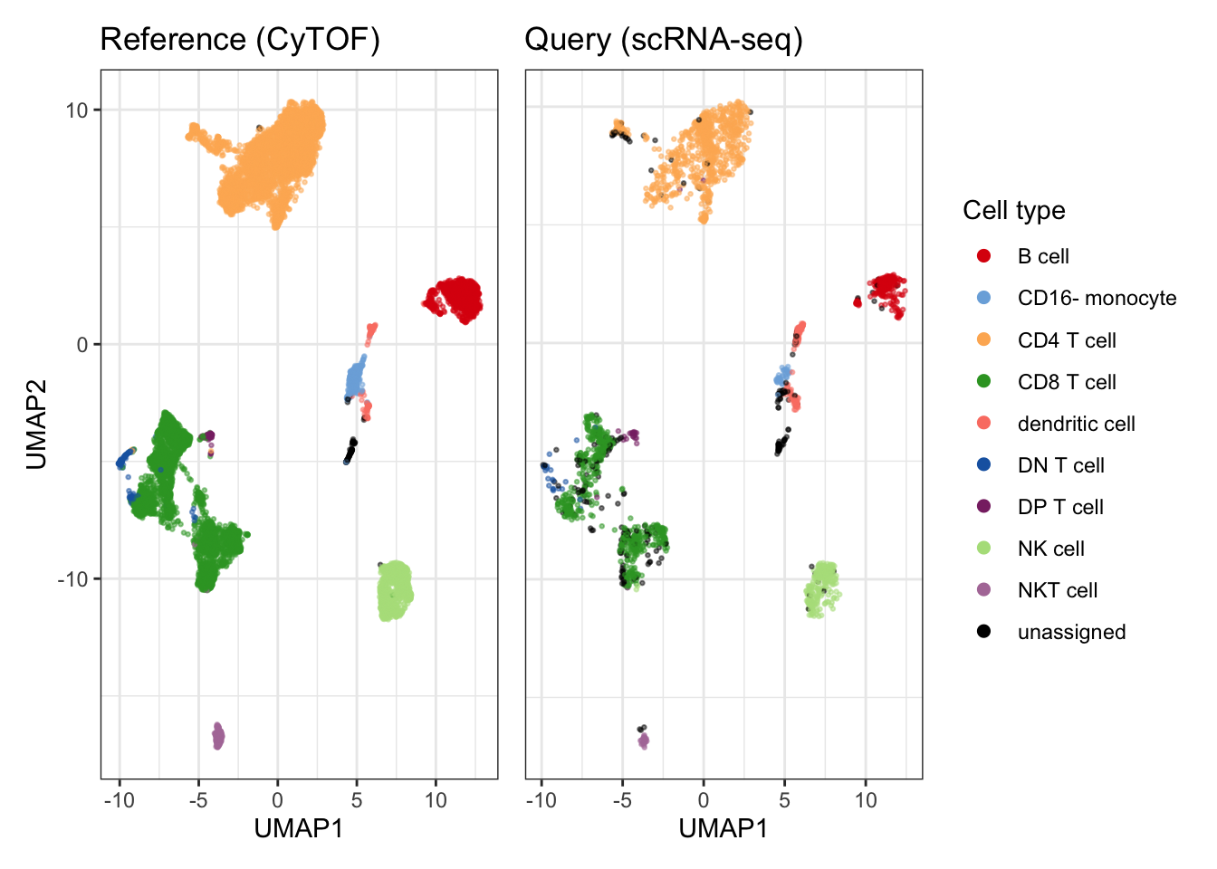
Figure 4B - Celltype abundances
library(ggplot2)
library(dplyr)
library(tidyr)
library(patchwork)
p_abundance <- plot_abundance_comparison(
  classified,
  ref_name = "CyTOF",
  query_name = "scRNA-seq",
  query_col = "predicted_celltype",
  CLR = TRUE)

# saveRDS(p_abundance, "results/05_cytof_rnaseq_abundance.rds")
# ggplot2::ggsave(p_abundance, filename = "figs/05_cytof_rnaseq_abundance.png")
p_abundance 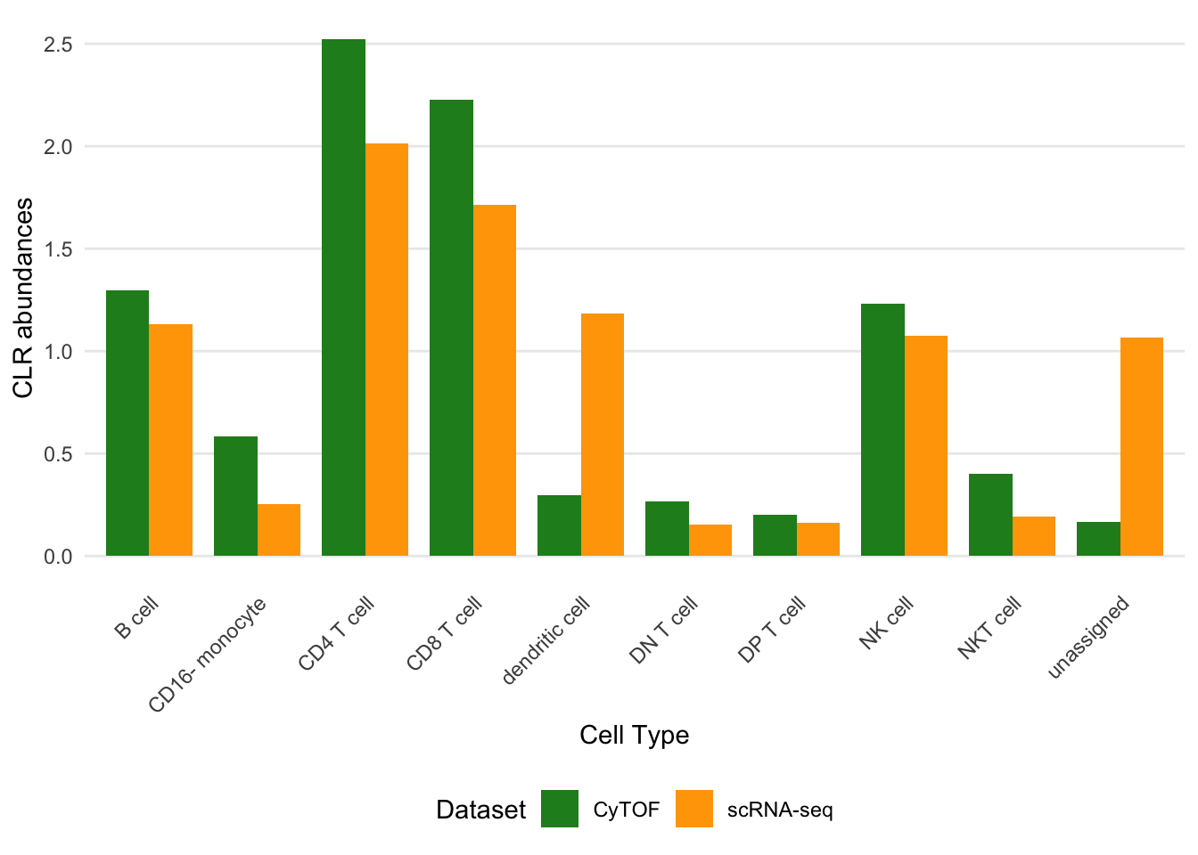
Figure 4C - Marker correlation
p_correlation <- plot_expression_correlation(classified, markers = markers, ref_name = "CyTOF", query_name = "scRNA-seq")

uncorrected$celltype <- c(as.character(classified$query$predicted_celltype), classified$reference$celltype)
p_correlation_raw <- plot_expression_correlation(uncorrected |> dplyr::filter(batch == "CyTOF"),
  uncorrected |> dplyr::filter(batch == "RNA"), query_col = "celltype", markers = markers, ref_name = "CyTOF", query_name = "scRNA-seq")

# saveRDS(p_correlation, "results/05_cytof_rnaseq_correlation.rds")
# ggplot2::ggsave(p_correlation, filename = "figs/05_cytof_rnaseq_correlation.png", height = 20, width = 20, units = "cm")
p_correlation
## `geom_smooth()` using formula = 'y ~ x'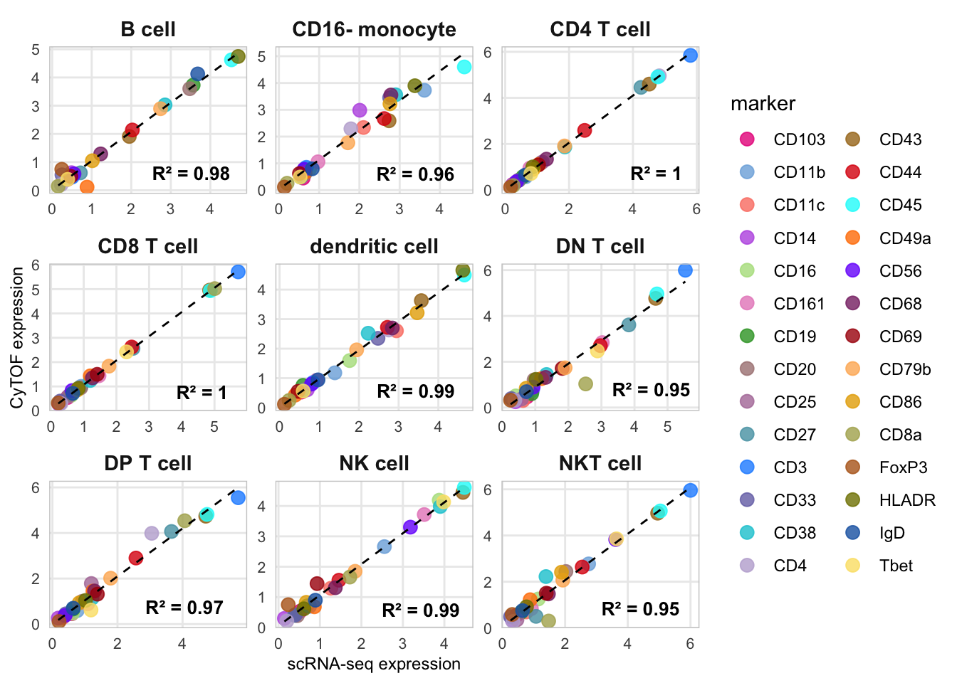
p_collected <- (( p_umap / p_abundance + theme(legend.position = "right")) | p_correlation ) +
  plot_layout(tag_level = 'new') +
  plot_annotation(tag_levels = list(c("A", " ","B","C")))

p_collected
## `geom_smooth()` using formula = 'y ~ x'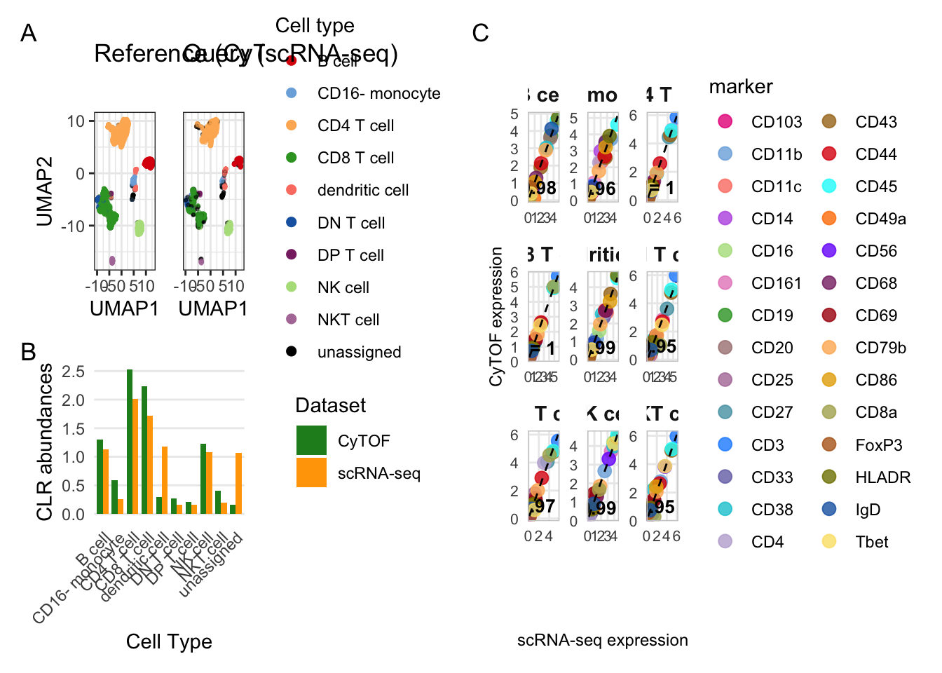
ggplot2::ggsave(p_collected, filename = "figs/05_cytof_rnaseq_abundance_correlation.png", height = 20, width = 35, units = "cm")## `geom_smooth()` using formula = 'y ~ x'Contact